Chi Squared Test

The Chi Squared Test is a statistical test that is often carried out at the start of an intended geographical investigation.

We may have noticed a pattern, distribution or anomaly in a feature of the human or physical world and have a hunch that ‘something is going on’ to produce it.

The Chi Squared Test tells us whether our ‘hunch’ is statistically significant – i.e. that – yes, we have noticed a valid geographical phenomenon that deserves further investigation as part of a geographical enquiry. Alternatively, it can indicate that what we think is a ‘phenomenon’ is actually just a random variation in the feature we’ve noticed, and doesn’t deserve further investigation or research.

So it’s a test to indicate: ‘There’s something valid going on here – investigate it further and work out what it is and what’s causing it’, or ‘Don’t waste your time – it’s just ‘chance’ or ‘random events’ that you’re seeing – move on and give your time to studying some other aspect of geography.

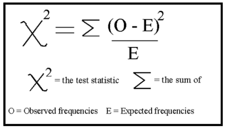
The equation compares what you have measured (Observed) in the distribution of the feature, against what may be anticipated (Expected) ‘if’ the feature was randomly distributed.

For the feature under investigation, establish a Hypothesis and then convert it to a Null Hypothesis

(Null Hypothesis: why do we need it? Well, in the investigative process it’s not possible to ‘prove’ something with 100% certainty – we only get to see and experience a part of the whole world, so it may be that what we think we’ve ‘proved’ in one place is ‘disproved’ in another. But we can ‘disprove’ assumptions 100% - by finding a contradictory occurrence of it.

We can never ‘prove’ a Hypothesis fully, but we can fully ‘disprove’ its converse – the Null Hypothesis. If our statistical tests allow us to disprove the Null Hypothesis then we can ‘accept’ that our Hypothesis has validity. But only to the extent that we can have ‘confidence’ that our sample is large enough and valid. This leads on to the concepts of ‘confidence levels’ and ‘critical values’ (below).

The Chi Squared equation

Chi Squared test example on coastal deposition

Imagine you were investigating the size of material deposited on a beach and noticed there were differences as you moved along the beach with pebbles seeming to become larger. You want to know if the variations in pebble size are significant or random. You have counted the number of pebbles over 5 cm long in a quadrat at 5 sites along a beach between 2 groynes. Is there a statistically valid variation?

Hypothesis: Beach material gets larger as you move south along the beach

Null hypothesis: there is NO significant variation in pebble size along the stretch of beach

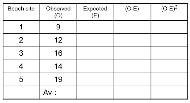
1. Step 1: put in the figures recorded in the Observed column (O)
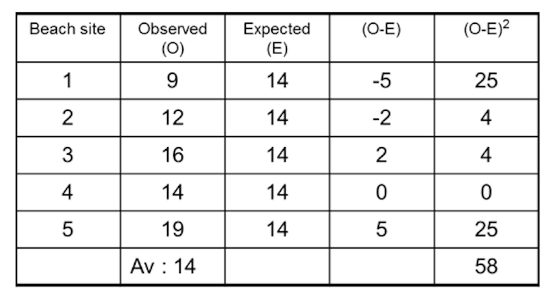
2. Step 2: work out the average (mean) figure for O (add up the column & divide by number of data sets)
3. Step 3: put the ‘average’ into the ‘Expected’ column (E)
4. Step 4: work out O-E and put into the next column
5. Step 5: work out O-E squared and put into the next column and total up the column
6. Step 6: that is the top part of the formula – now divide by the ‘E’ figure to get your chi-squared number

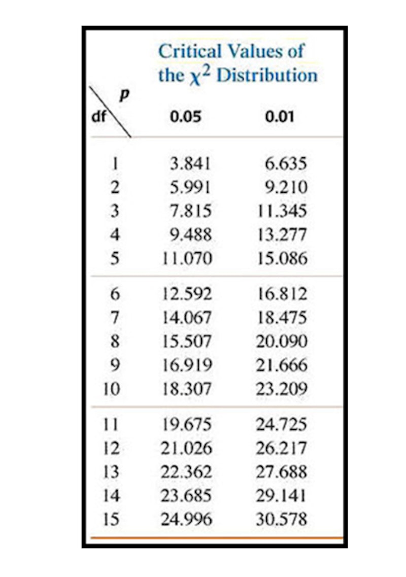
On its own the Chi Squared statistic has little meaning – it needs validating against ‘critical values’. These are found in tables or on graphs that have been calculated by statistical experts.

Consider what ‘confidence level’ you wish to use. The most common levels in geography are 95% and/or 99%. These mean that 95 out of every 100 times you carried out these measurements (or 99 out of 100) you would get a similar result, but on 5 occasions (or 1) you may get ‘chance’ results.

They may be expressed in a range of ways:

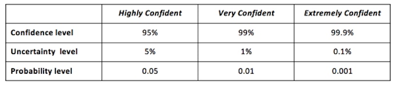
The second factor, after Confidence Level is the ‘Degrees of Freedom’ (df) to use. This is usually calculated as n-1 (number of data sets minus 1) which in this example is 5 (beach sites) -1 = 4. So we use the df 4 row to look up our ‘Critical Value’.

(Degrees of Freedom is a complicated statistical feature that it is not necessary to understand for A level Geography other than to know how to use. If you’re interested, it’s the number of values in the final statistic that are allowed to vary. No… nor me either!)

The table shows ‘Critical Values’ that have been calculated by statistical experts that we judge our Chi Squared result against. If our result is larger than the Critical Value – we have got a valid result in our data that lets us reject the null hypothesis and accept our original hypothesis. It our result is smaller than the Critical Value, we have to accept the null hypothesis – that there is no key geographical process observable in this data set.

Step 7: Looking at the Critical Values table at df 4, we can see that our Chi Squared result of 4.14 is smaller than the 9.488 of the 0.05 probability (95% certainty) so we have to accept the null hypothesis that: there is no significant variation in pebble size along this stretch of beach.

Is that the end of it?

Well – it might be that our sample size is too small and if we were still convinced that beach material varied along the coast we should consider collecting data on more pebbles at more sites. And maybe our choice of 5cm as the key measure should be altered to other criteria. But for the data we collected, at those five sites, there is not enough variation in the data to be sure that it is not just random beach accumulations that we have noticed and recorded.